Understanding the g-factor in SENSE Reconstruction
Contents
SENSE (Sensitivity Encoding) accelerates MRI by undersampling k-space, causing aliasing where signals from distinct locations ($r_1, r_2, \dots, r_R$) overlap onto a single pixel $r_p$. Coil sensitivities are used to unfold these signals.
SENSE Unfolding & Noise (R-fold Undersampling)
For $N_c$ coils and an acceleration factor $R$, the measured aliased signals $\mathbf{m}_{\text{aliased}}(r_p) \in \mathbb{C}^{N_c}$ at pixel $r_p$ are:
Where:
- $\mathbf{m}_{\text{true}}(r_p) = [m(r_1), m(r_2), \dots, m(r_R)]^T \in \mathbb{C}^{R}$ are the true image intensities at the $R$ aliasing locations.
- $\mathbf{S}(r_p) \in \mathbb{C}^{N_c \times R}$ is the sensitivity encoding matrix for pixel $r_p$:
with $S_c(r_k)$ being the sensitivity of coil $c$ at location $r_k$.
- $\mathbf{n}(r_p) \in \mathbb{C}^{N_c}$ is the noise vector.
Reconstruction involves inverting $\mathbf{S}(r_p)$ (typically via pseudo-inverse if $N_c > R$):
where $\mathbf{S}^{\dagger} = (\mathbf{S}^H \mathbf{\Psi}^{-1} \mathbf{S})^{-1} \mathbf{S}^H \mathbf{\Psi}^{-1}$ and $\mathbf{\Psi}$ is the noise covariance matrix. If noise is i.i.d. with variance $\sigma_n^2$ across coils, $\mathbf{\Psi} = \sigma_n^2 \mathbf{I}$.
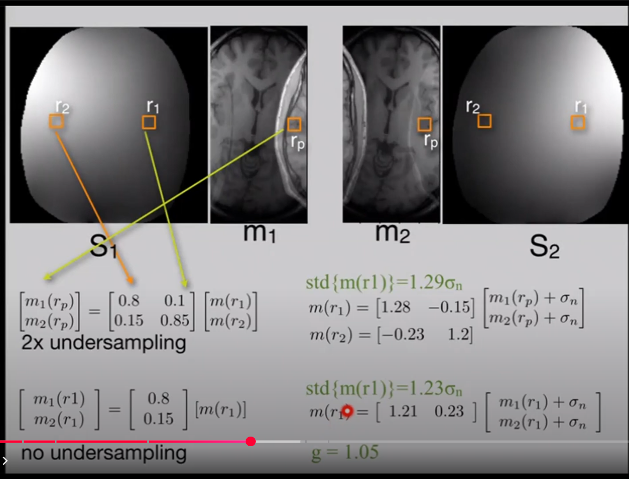
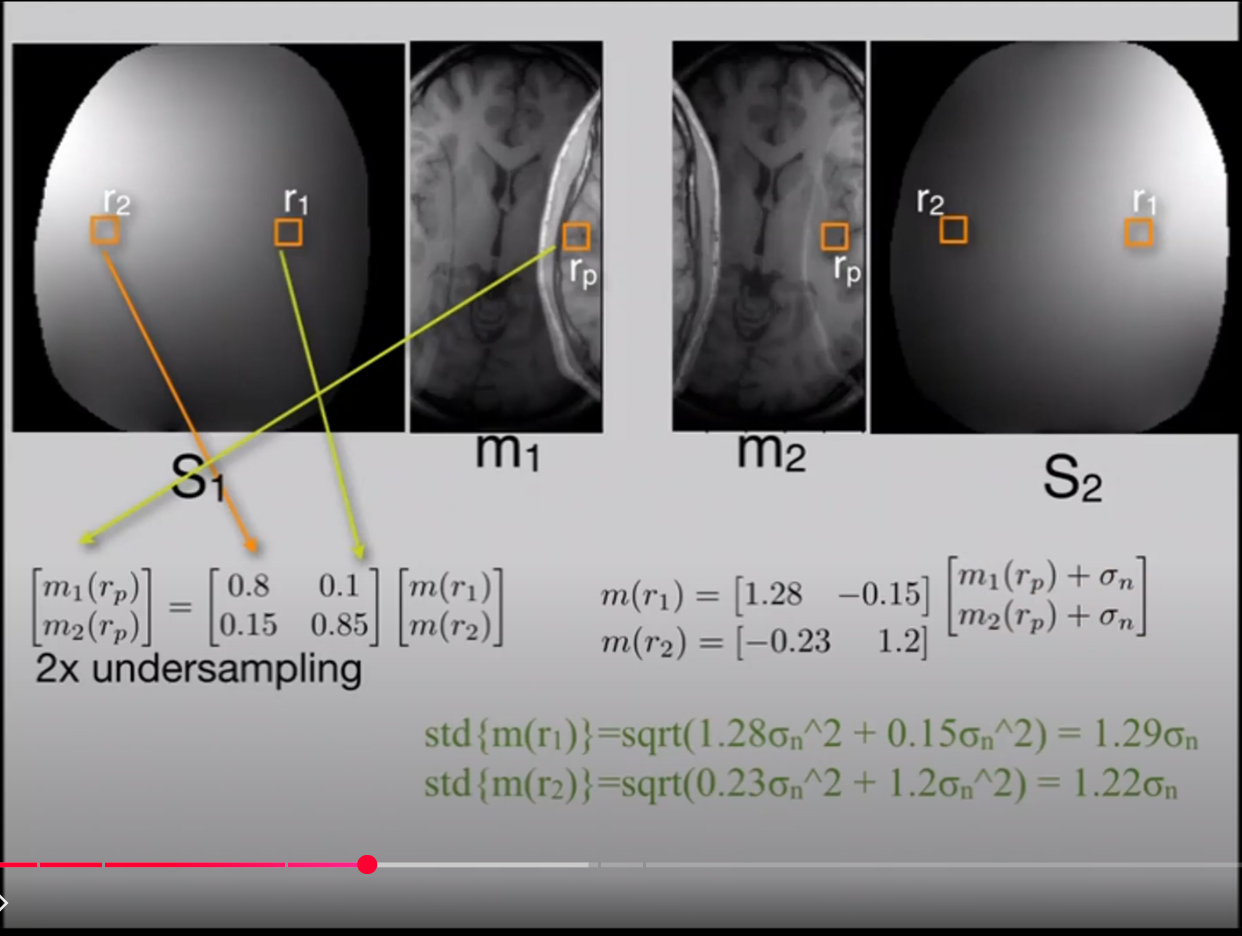
Example (R=2, $N_c=2$, i.i.d. noise):
If $\mathbf{S} = \begin{bmatrix} 0.8 & 0.1 \ 0.15 & 0.85 \end{bmatrix}$, then
$\mathbf{S}^{-1} = \begin{bmatrix} 1.28 & -0.15 \ -0.23 & 1.2 \end{bmatrix}$.
The g-factor
The g-factor at a specific unfolded pixel location $r_k$ quantifies noise amplification due to the unfolding process (for undersampled SENSE) or coil combination (no undersampling).
The noise covariance of the unfolded image $\mathbf{m}_{\text{true}}$ is:
If noise is i.i.d. in raw coil data ($\text{cov}(\mathbf{n}) = \sigma_n^2 \mathbf{I}$), then:
The standard deviation of the $k$-th unfolded pixel $m(r_k)$ is:
The g-factor for pixel $r_k$ is often defined as:
A common simplification when $N_c=R$ and noise is i.i.d. per aliased pixel measurement:
If
and each element of $\mathbf{m}_{\text{aliased}}$ has noise std $\sigma_n$:
Then:
Example (R=2, $N_c=2$, using $\mathbf{S}^{-1}$ above):
- $g(r_1) = \sqrt{ (1.28)^2 + (-0.15)^2 } \approx 1.29 \implies \text{std}{m(r_1)} \approx 1.29 \sigma_n$
- $g(r_2) = \sqrt{ (-0.23)^2 + (1.2)^2 } \approx 1.22 \implies \text{std}{m(r_2)} \approx 1.22 \sigma_n$
No Undersampling (Full FOV, R=1)
Signal equation for pixel $r_1$ with $N_c$ coils:
where $\mathbf{m}(r_1) = [m_1(r_1), \dots, m_{N_c}(r_1)]^T$ and $\mathbf{s}(r_1) = [S_1(r_1), \dots, S_{N_c}(r_1)]^T$.
Optimal combination (assuming i.i.d. noise $\sigma_n$ per coil):
The variance is:
The g-factor is:
Often, $g \approx 1$ for no undersampling, reflecting optimal coil combination. Example value $g=1.05$ might account for practical factors or a different noise reference.
Interpretation & Influencing Factors
- $g \approx 1$: Minimal noise amplification
- $g > 1$: Noise amplified, local SNR reduced. $\text{SNR} \propto \frac{1}{g\sqrt{R}}$
Factors influencing g (SENSE):
- Coil Geometry: Distinct sensitivity profiles $\implies$ lower $g$
- Acceleration Factor (R): Higher $R \implies$ generally higher $g$
- Pixel Location: $g$ is spatially varying
- Regularization: Can affect effective $g$
Lower g-factors are desirable for better image quality.
Author MyBlogTestAuthor
LastMod 2025-12-23